Wolfram Winter School 2022 Guest Lecture

Hi everyone,

This past winter, I was invited to give a guest lecture at the Wolfram Winter School. Below, I have posted a recording of my talk!

I present an overview of the research which has grown out of the project I completed for the Wolfram Summer School in 2020. The talk touches many fields of computational science, as this type of simulation has quite broad applicability. The central results relate to our study of hard sphere systems, and in particular the construction of the hard sphere causal graph.

I hope that you enjoy! It’s a bit of a long journey, but there appeared to be at least some people who stuck it out until the end and found it valuable!

Cheers,

-Matt

Functional Derivative Cheat Sheet

(Update: LaTeX version of the cheat sheet available for download!)

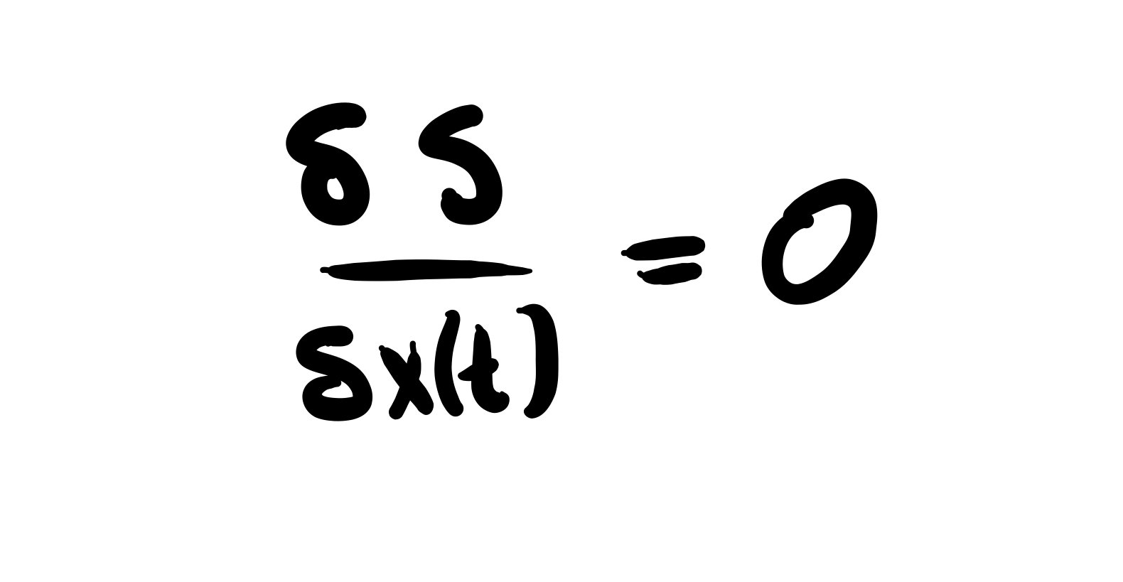
I’ve been rather perplexed at how difficult it is to find good information about functional derivatives on the internet. Many, many textbooks discuss variational calculations––for example, the principle of least action––using what’s called the total variation of a functional:

These are extensively documented (see, e.g., Boas, Mathematical Methods in the Physical Sciences) and so I will not discuss them further here.

However, often in physics one often comes across expressions such as this:

These “functional derivatives” are very similar to the total variation above, but for some reason I have had a much harder time finding good information about them online. When they are discussed, they are often simply treated using the total variation.

However, this is a perfectly well-defined derivative, and it is often quite convenient (and conceptually simpler) to use this form. For this reason, I have thrown together a cheat sheet of functional derivative identities (including the definition, boxed in blue) which are quite useful.

These are all derived carefully here, including many worked examples. But for quick use, I think this will be valuable to people!

Cheers, and happy differentiating!

-Matt

Exploring the Central Limit Theorem Computationally

Hello everyone! Welcome to Stochastic Tinkering :)

Today, I would like to write a bit about the Central Limit Theorem.

I have taken several courses in the past in which I was taught the Central Limit Theorem, but it has never quite made sense to me. However, in a conversation with Stephen Wolfram at the 2021 Wolfram Summer School, Nassim Taleb provided a Mathematica demonstration which allowed me to understand the Central Limit Theorem better than I ever have before. In what follows, I have tried to reproduce what I was able to understand from Dr. Taleb’s presentation. All credit for brilliance goes to Dr. Taleb, and all errors are my own.

I hope that you will find the demonstration as valuable as I did.


Roughly speaking, the Central Limit Theorem says that sums of independent, identically distributed random variables will themselves tend to be normally distributed, regardless of the underlying distribution of the random variables. When stated like this, I have to think very hard to understand what the CLT is actually saying. But Taleb’s demonstration makes things much clearer.

First, let’s get some random variables. We’ll start with a uniform distribution on the interval [0, 1].

1.png

This is what is meant by “independent, identically-distributed random variables.” We are just sampling our distribution over and over again, and we end up with a bunch of values between zero and one. Now, we sum them up. In this case, the sum is equal to 44.9921.

We do not have any reason to care about the particular value of 44.9921 by itself. However, a pattern emerges if we repeat this procedure above many times and compare the results.

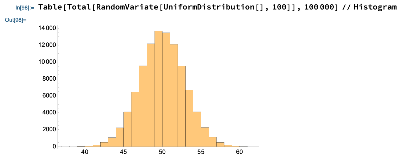
Evidently, the answer tends to be around 45-50ish, but it fluctuates each time we run the computation. To understand the fluctuations, let’s repeat this procedure a large number of times, and look at the histogram of our results.

3.png

That’s a Gaussian! And that is the Central Limit Theorem: sums of random variables tend to form a normal distribution when you run the experiment many times. But if this verbiage is confusing, just look at the Mathematica code! That one line contains the heart of the CLT.

People tend to discuss the CLT in terms of averages of the random variable being sampled. But of course, if a sum of random variables is normally distributed, so too will be the average––the average is proportional to the sum!

4.png

The only difference is that now we have replaced “Total” with “Mean”. We see a gaussian yet again––a different mean and a different variance, but a gaussian all the same.


Let us now poke and prod at this result from various angles. How robust is it? We made a few choices above. Does this central-limiting behavior depend on any of those choices?

Firstly, we decided to sum up 100 random samples. What happens if we change this number? Let’s use 2, 3, 5, 10, 1000, and 10000 samples, and see what happens.

5.png

Evidently, two random samples is not quite enough to get the gaussian distribution. But even with three samples, the distribution is clearly taking shape. So central-limiting behavior appears to be robust to the number of random variables summed.

We also arbitrarily decided to run the experiment 100,000 times and plot a histogram of the results. How does central-limiting behavior depend on the number of trials? We expect that we need a certain minimum number of trials to even know what shape the distribution takes. Let us try powers of 10: 10, 100, 1 000, 10 000, 100 000, 1 000 000, 10 000 000. (We now return to using 100 samples).

6.png

Perhaps this is what we should have expected! Below a certain number of trials, it is not at all clear what the distribution will ultimately look like. But around 1000-10000 trials, the distribution is clearly taking shape.

We conclude that above a certain minimum number of samples and trials, we can expect central limiting behavior to emerge, at least for the uniform distribution.


So let us finally turn to the most interesting variable in our experiment: the statistical distribution being sampled. We originally chose a uniform distribution on the interval [0, 1]. What happens when we choose other distributions? As it turns out, some distributions converge much more slowly to central-limiting behavior.

Suppose, to test the dumbest case first, we sample instead from a normal distribution. We would certainly hope that the sums of these random samples are distributed normally. And indeed this is what we observe.

7.png

How about discrete distributions? The Bernoulli distribution describes events with only two possible outcomes, one of which has probability p and the other (1 - p). This distribution might describe the outcomes of flipping a (potentially biased) coin. If p = 0.75 and we flip 10,000 coins, we might see a distribution like this.

8.png

Does the Bernoulli distribution exhibit central-limiting behavior? It is easy enough to test.

9.png

Indeed it does! So the CLT is clearly at least a somewhat robust phenomenon to the choice of statistical distribution.

Now, let’s break it.


To do so, we will use fat-tailed distributions, which Taleb has written about extensively in the Incerto. One example of a fat-tailed distribution is the Pareto distribution, which has a power-law tail.

11.png

We can see that for α ~ 1, the tail of this distribution does indeed get long. What does this mean for our samples? Let α = 1.2, which appears to be close to the edge separating fat vs. thin-tailed. We sample this distribution a large number of times.

12.png

At first, this seems like a boring histogram with all data concentrated near 0, but if we look closer, we can see that 1 of our 1,000,000 random samples exceeded a value of 10,000! Perhaps you can already see why fail-tailed distributions are a problem for the central limit theorem.

Let’s run our usual experiment again on the Pareto distribution.

13.png

That’s not a gaussian! It appears that we get nearly 1,000,000 results clustered near 0, and yet a very small number of sums, just 70, exceed 20,000!

So we can already see that fat-tailed distributions are a different beast. With this number of trials and samples-per-trial, central-limiting behavior had already emerged in every other distribution we have look at thus far. Let us see if increasing both of these numbers allows us to get closer to the normal distribution we expect. Let’s try increasing the number of samples to 10,000 and the number of trials to 10,000,000.

It appears that things are not getting better: we are still nowhere close to the Gaussian we were hoping for! And my computer is really starting to sweat. So, when α is below a certain value, the Pareto distribution does not exhibit central limiting behavior––at least, not without a very large amount of computation. Is this very slow convergence to central-limiting behavior a particular property of the Pareto distribution?

Another fat-tailed distribution is the Cauchy distribution. We determine whether the Cauchy distribution exhibits this same property.

14.png

Although the distribution looks bell-shaped, in fact the formula for the PDF is given by

15.png

and hence it decays much less quickly with x than the Gaussian does. Let us now perform our central limit test again.

Again, this is nowhere close to a gaussian, even having sampled 10,000,000 times! Almost every sum is approximately zero, except for the one that exceeds 60 million! (With a few in between.)


I could continue along these lines, but I think that the central message should by now be clear. The CLT is a real phenomenon. Central-limiting behavior emerges robustly from a wide variety of statistical distributions––discrete, continuous, finitely supported, infinitely supported––after a non-astronomical number of trials. It is easy to observe this behavior with small computational experiments run on a laptop.

However, there exist distributions that do not practically obey the Central Limit Theorem. These distributions, fat-tailed distributions, have the property that there is a non-negligible (but still small) probability of generating a sample with a very large magnitude. In fact, I believe that these distributions do exhibit central-limiting behavior eventually, but our explorations have revealed that we would need astronomical numbers of trials before we observe this behavior.

The Central Limit Theorem is widely used for statistical inference––for example, when using a sample mean to estimate a population mean. It is thus heartening to know that we can reliably reproduce central-limiting behavior in controlled computer experiments under rather general circumstances. Nevertheless, in real-world experiments, if there is reason to believe a variable is fat-tailed, other techniques will probably have to be used for reliable inference.


I hope that you have found this demonstration illuminating! I certainly learned a lot while exploring these ideas. I should also recommend for the nth time that you read Dr. Taleb’s books.

Thank you for coming to my blog, and I hope I will see you back here soon :)

Until then, be well.

-Matt

Simulating Flocks of Birds

Hi there!

This post is a copy of my final project for my Statistical Physics of Living Systems course. It is a summary of the self-propelled particle computer simulation technique, with an application to modeling a flock of birds.

(I apologize for the graininess as it is currently presented. If this bothers you, here is the original PDF.)

Also, here is a video of one of the simulated flocks.

Finally, here is the code, if you want to make animations yourself.

I hope you enjoy :)

Sincerely,

-Matt

1.png
2.png
4.png

Everyone to Everyone

“The fundamental property of the internet, more than any other single thing, is that it connects everyone to everyone.” - Naval Ravikant.


Hello everyone! Welcome to my blog :)

Today, I have a quick back of the envelope calculation to share with you, which has a somewhat surprising result.

Here’s the basic question: how many collaborations between people could the internet possibly facilitate? I was inspired by this quote from Naval Ravikant above to look into this question. The combinatorics are quite straightforward, so it’s not hard to get a numerical answer.

Assumptions: Let’s assume that everyone on Earth has access to the internet. We’ll call the total population P ~ 8 billion. Furthermore, we’ll assume that everyone can, in principle, contact everyone else who is connected to the internet. (Recall, this is a back of the envelope calculation. All models are wrong, some are useful!) We will define a collaboration to be a group of two or more people.

Let’s dive into it.


We’ll do some concrete calculations to get started. How many collaborations are possible between two people on Earth? We can guess that the answer is going to be something like “a lot.” The way you compute it is

IMG_18E1BDF2D2E9-1.jpeg

where “C” is the number of collaborations. Why? Well, there are P choices for the first person in the collaboration, and P-1 choices for the second. We divide by two since (you, me) is the same collaboration as (me, you). Plugging in numbers, we see that

IMG_E0D482102DFD-1.jpeg

So there are about 10^19, or 10 quintillion possible two-person collaborations that the internet makes possible. That’s already an enormous number. So how about collaborations of three people?

IMG_BF8406CE4DD1-1.jpeg

or 100 octillion. So there are 10 billion times as many three-person collaborations as there are two-person collaborations! These numbers are already ridiculously large, which is just a hint that our total answer is going to be dominated by larger collaborations.

(Why the 6 in the denominator? It’s how many ways you can rearrange/permute a set of 3 objects. Recall that we do not want to count (me, you) differently from (you, me). )


The general formula for the number of collaborations between M people is given by

IMG_2A7BD3C209BC-1.jpeg

which is known as the “binomial coefficient.” The exclamation marks refer to factorials. The term P!/(P-M)! will give us P(P-1)(P-2)…(P-(M-1)). The M! in the denominator ensures that we do not count any collaboration multiple times by permuting its members.

We have already seen

IMG_D50B8A95117F-1.jpeg

But now that we have a general formula, we can start moving towards answering our initial question. First, we should realize that the total number of possible collaborations will be (the number of two-person collaborations) + (the number of three-person collaborations) + … , so we are actually interested in the quantity

IMG_CA3CC5218952-1.jpeg

Let’s get a feel for the types of numbers involved here. Let’s say, for instance, that you wanted to see how many ten-person startups the internet could possibly facilitate. The answer would be

IMG_EC1966349E3A-1.jpeg

or 100 novemvigintillion. (Okay, that name is probably not particularly useful to include, but have you ever heard before?? Me neither.)

It is probably worth remembering that the number of atoms in the universe is only ~ 10^79, so there are 10 trillion times the number of possible 10-person startups as there are atoms in the universe. This is number is literally astronomical! And remember that we are going to consider collaborations up to 8 billion people, so we’re really just getting started.

What if you wanted to start a 100-person message board to share old southern pie recipes? Well then, you could construct

IMG_C3E1A144DFB7-1.jpeg

such message boards. We’re now firmly beyond the territory where our imagination can be helpful. This number is stupidly large.

Or suppose you wanted to put together a mailing list to distribute your Space-Is-Fake conspiracy newsletter to 10,000 devoted followers? Then you could construct

IMG_CFE059531E92-1.jpeg

such mailing lists. Okay, we’re just having fun at this point, but these calculations are really starting to make Mathematica sweat. There is no hope for us to put 8,000,000,000 as the upper bound for that summation and have the computer spit anything out before we’re old. So what can we do?


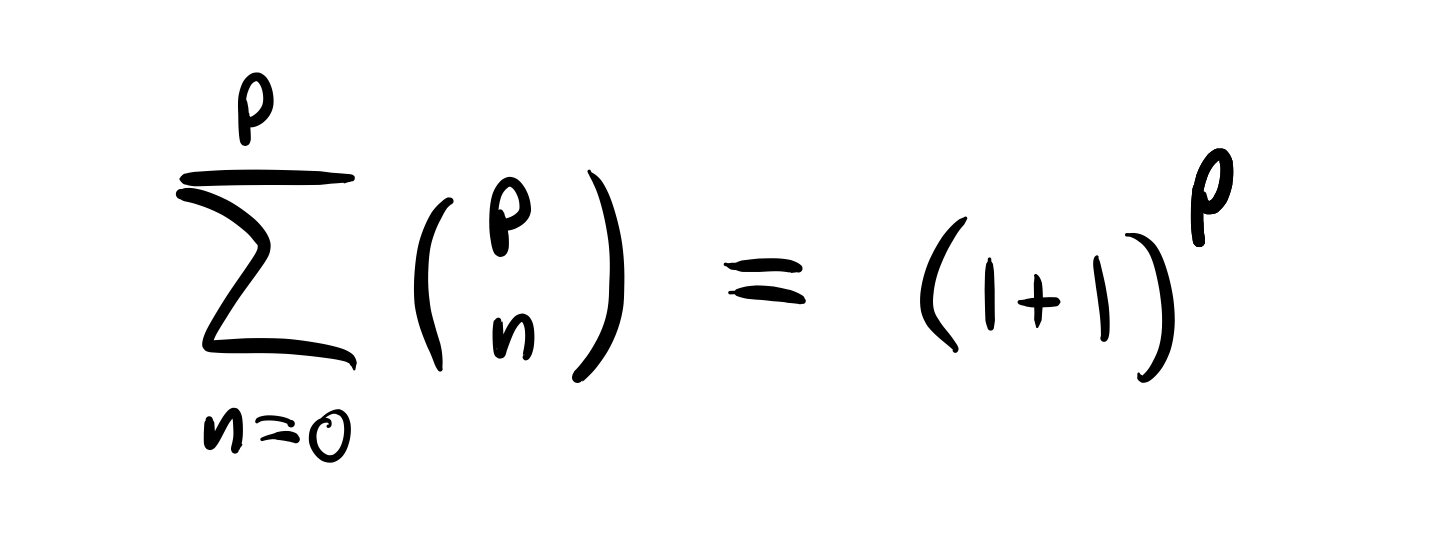
Well, there is a very useful result in math involving the binomial coefficient which is known as the binomial formula:

IMG_28D9A02E8CC3-1.jpeg

In general, this is a useful result for expanding out polynomials. But x and y are simply numbers, so look what happens when we plug in x = y = 1:

IMG_98BC1D1DD635-1.jpeg

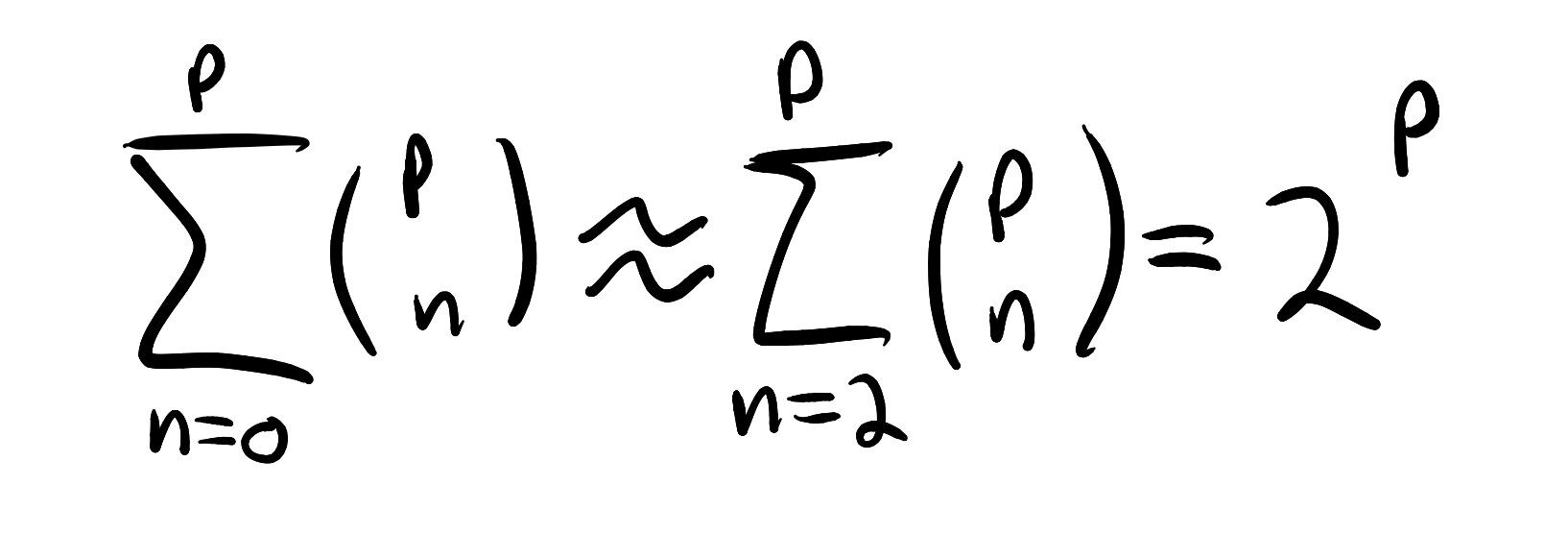
Or, in other words,

IMG_A99F998C8239-1.jpeg

where we have only made the small approximation of omitting the first two terms of the sum.

But this final equality is precisely what we want! It tells us how to compute the total number of possible collaborations involving at least two people. Plugging in numbers, we get

IMG_2FB49534D5F2-1.jpeg

Take a good look at that last number. Unless you regularly watch Numberphile (which you should certainly do), I can almost promise that that is the biggest number you have ever seen.

In summary, how many collaborations could the internet possibly facilitate, in principle? Well, 10^(30 million) or so.


But why is any of this important? I sincerely believe that there is more to this post than me just writing down very large numbers, and saying “look how ridiculously, gobsmackingly large that number is!”

Because that number of 10^(30 billion) is more than an idle mathematical result. It suggests the potential of the new world that has opened to us with the advent of the internet. Although the everyone-to-everyone approximation that I made to perform these calculations is a bit unrealistic, it gets less so with each passing year. And I believe that this was Ravikant’s point in the quote at the top of this post.

Whether we have realized it or not, the internet has opened up access to a combinatorially enormous space of possible projects, collaborations, businesses, groups, and friendships. We spend a considerable amount of time at one another’s throats, but if we could stop and take stock for a moment, perhaps we would see the universe of possibilities that awaits us at our fingertips at all times.

Think of the technologies that could be found by even partially mining this space of collaborations. The art. The science. The love. The wealth to be found for us all, especially those who need it most.

Sometimes I find it hard to imagine that the future will be good. It can be hard to see where we can go from here as a species. But this little exercise is actually helpful check on that pessimism. I’m not saying that we will necessarily maximize our potential, but there is plenty of room up there for us to get started :)

Thanks for reading my blog!

-Matt

P.S. I originally heard the Ravikant quote in this Meaningwave song by the inimitable Akira the Don.

HardSphereSimulation[]

Hello everyone,

This is just a quick post to draw attention to my first contribution to the Wolfram Function Repository: HardSphereSimulation. It is a function which simulates the evolution of a non-dissipative hard sphere gas/liquid in an N-dimensional box with reflecting boundary conditions. I am currently exploring the thermodynamics of such systems for my research. Here is a fun little preview of its functionality:

FrictionlessPool.gif

-Matt

Percolation

Hi everyone!

Welcome to my blog. I think I’ve got something very cool for you today. It’s a model from theoretical physics known as percolation, and it involves structures that look like this:

p%3D0.5.jpg

Let’s get into it!


The Question: Can you predict whether fluid will flow through some porous substance?

The Model: Consider an infinite grid of pairs of integers. With probability p, connect a point in the grid with one of its nearest neighbors (excluding diagonals), and otherwise do not connect them. Repeat this process between all adjacent pairs of points in the grid. If two points are connected by an edge, we say that fluid can flow between them. Otherwise, fluid cannot flow. Having done this, you will have a random graph whose appearance will depend on p. We will say that fluid can flow macroscopically through this substance if, somewhere in our infinite grid, there is an infinite cluster of connected points.

To make things concrete, first let’s take a look at the grids.

SampleGrids.png

As you can see, the value of p (know as the porosity parameter) controls the number/density of connections on the graph. Recall that we are imagining that fluid can flow along the connections between the “pores.”

Just by eye, we can see that fluid could certainly flow through the grid when p = 1, and it certainly could not flow when p = 0.25. It seems likely as well that fluid could flow when p = 0.75, although perhaps not certain. How about p = 0.5? This case is significantly less clear.

The requirement for fluid to flow on “macroscopic scales” is that there needs to be some cluster (i.e. a connected region) that has an infinite number of nodes when our grid extends off to infinity. Let’s take a look at the behavior of clusters.

Clusters.png

These are the five largest clusters for a random grid with p = 0.4. For this value of p, none of our clusters extends more than half way across the grid. It therefore seems unlikely that we will find an infinite cluster as we extend our grid farther out. Let’s see what happens at p = 0.5.

CriticalValue.png

Here, we have a slightly different story. Now the cluster has extended all the way across our grid. To make sure this isn’t a fluke, let’s see what happens on some larger grids.

CriticalValue2.png
CriticalValue3.png
CriticalValue4.png

So what’s the verdict? Will fluid flow at p = 0.5? Somehow, it still feels uncertain. It seems to cross these 40x40 grids most of the time, but an infinite grid is a different animal. Could one of those clusters really extend to infinity at this level of connectivity?

Well it turns out that it is possible to prove that there cannot be an infinite cluster for p = 0.5. However, it is the case that p = 0.5 is a very special value for this model because the system actually experiences a phase transition at p = 0.5. What this means is that for all p < 0.5, no fluid can flow macroscopically on any such random grid (i.e. there can be no infinite clusters). Moreover, for all p > 0.5, fluid can flow macroscopically on all random grids. In fact, it is possible to prove that there will be exactly one infinite cluster for all random grids with p > 0.5.

Such a discontinuous transition between “impermeable” and “permeable” is surprisingly rich behavior for such an apparently simple model!


However, this is not the end of the surprises to be found in the percolation model. People also study variants of the model in higher dimensions, and variants of the model where the “sites”/nodes are randomly populated instead of the “bonds”/edges. Each of these variants presents its own interesting behavior and subtleties.

It is also known that this system exhibits universality at the phase transition. I am not very familiar with universality, but what little I understand suggests that it is a truly fascinating phenomenon. Systems that exhibit universality have macroscopic properties which do not depend sensitively on the details of the underlying physics and instead only depend on the dimension of space. One consequence of universality is that vastly different systems may behave in similar ways during phase transitions.

However, I will say no more, because I am now out of my depth yet again!


Unfortunately, as you probably have noticed, all I can do is quote results and run small simulations here. Percolation theory is apparently quite technical to explore analytically, and I have been getting my information for this blog post from The Princeton Companion to Mathematics (which is an excellent and approachable book, by the way).

I hope that in the future I can learn more about the physics of percolation models. If I learn anything cool, I promise you guys will be the first to know :)

Thank you for visiting my blog!

Until next time, be safe and be well.

-Matt

Infinisecting & Exotic Shapes

Hello everyone,

I wanted to share with you a quick math puzzle today. I had fun working it out, and maybe you will enjoy looking at it. I hope that maybe someone else decides to try this because it seems like there could be an enormous diversity of solutions to this puzzle, and I could only really come up with a few! (Please leave any solutions you come up with in the comments!)

Puzzle: Construct a compact shape in two dimensions such that, if you cut through the shape in a straight line, you divide it into an infinite number of pieces. Let us call this cut an “infinisection” of our shape.

To get a feel for what I’m talking about, consider the following simple examples. We can trivially divide a compact line segment and a circle into two pieces by cutting through each with a straight line:

Example1.jpeg
Example2.jpeg

It is also not difficult to conceive of shapes which could be cut into a very large number of pieces:

Example3.jpeg

You could imagine extending this for 100 miles. Or a million. So long as you stop somewhere, since the shape just must be compact. But since we are stopping somewhere, shapes like this will always be cut into a finite number of fragments.

So again, the puzzle is to come up with some compact shape such that if we apply the procedure above, it is cut into an infinite number of pieces. Intuitively, it seems like such a shape is going to have to do a lot of oscillating or folding or doubling back on itself if it is going to fit an infinite amount of waving in a finite space.


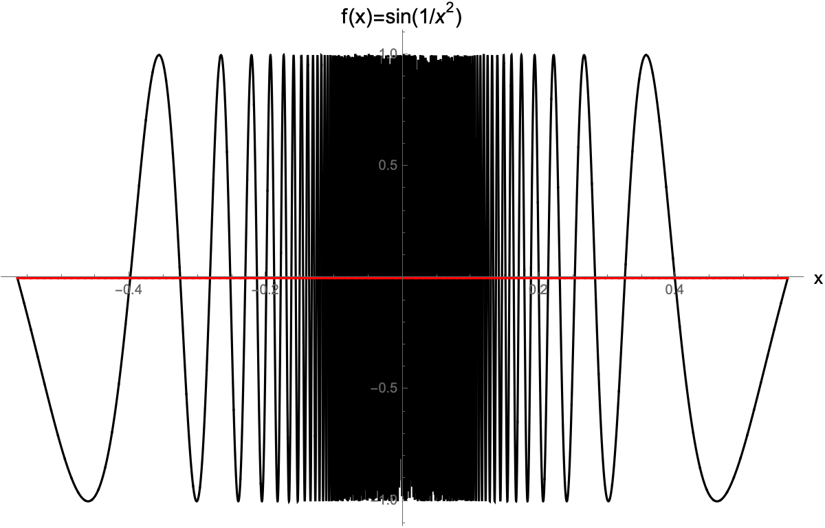
And in fact, we can construct a solution by looking for examples of things that oscillate an infinite number of times within a finite space. One such shape is the curve traced out by the function

sin.png

The zeros of this function occur when

Roots.jpeg

(restricting ourselves to the reals). We must truncate the curve somewhere to ensure the compactness of the shape. Without loss of generality, we truncate the curve at ±x1 = ±1/sqrt(pi). Does this curve in fact oscillate an infinite number of times between the endpoints we have specified? Yes!

Sequence.jpeg

Since there is an infinite number of natural numbers n, there will be an infinite number of xn’s in our interval.

Now that we have a curve which oscillates an infinite number of times in a finite space, it is simple to choose a line that infinisects it: simply choose the line f(x) = 0. That way, the curve gets cut at each of its zeros, and the pieces are the nonzero parts of the function between those zeros!

CutSine.png

Well, there we are. This is at least one example of a compact shape that can be cut into an infinite number of pieces with a straight line. Can we construct others?


Yes, it is actually not too difficult to do so. We can use many functions and curves that have some periodicity to them to accomplish what we accomplished above. We could imagine making trivial changes to the curve above which preserve its essential structure:

DecayingSine.png
SquaredSine.png
ExpSine.png
AsymmetricExpSine.png

So, once we have one solution, it is fairly easy to construct an arbitrarily large number of other solutions. However, none of these is really more interesting than the original.

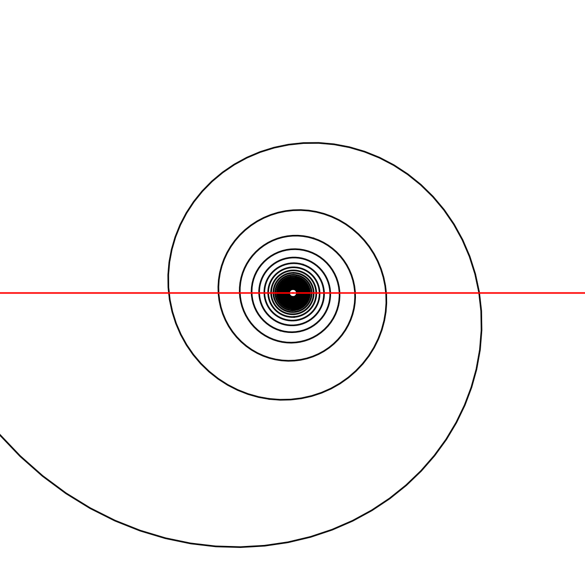
A slightly more interesting example is that of an asymptotically decaying spiral

Spiral.png

which we could parameterize with something like

SpiralCurve.jpeg

This is a bit unsatisfying since we have in some sense made our shape non-compact in its parameterization (i.e. t is unbounded), but we can prove that does the job all the same.


So far, we have found many shapes which can be infinisected by straight line. However, all the shapes that we have considered above have been highly regular: they each essentially have some periodicity and some asymptotic acceleration which allow them to fit an infinite curve into a finite amount of space. But I can’t think of any reason why there shouldn’t be just as many––probably far more––irregular shapes which also solve our puzzle. This is where the puzzle gets much more interesting, and far harder. Beyond this point I can only make educated guesses.

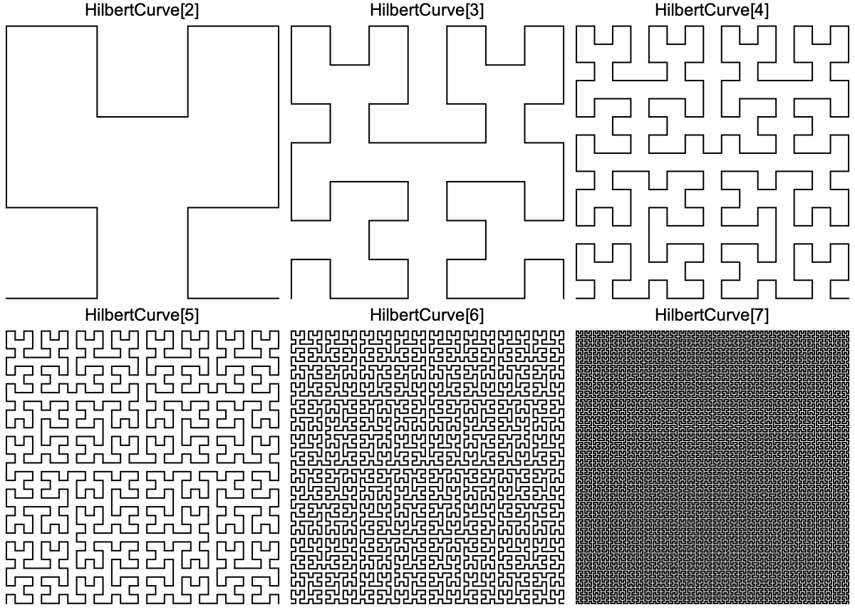
We may be able to construct one such “irregular” example from a space filling curve such as a Hilbert curve. A Hilbert curve is a continuous one-dimensional curve which weaves through space in such a way that it touches every point in some two-dimensional region exactly once. It is constructed by taking the limit of curves which look like this:

HilbertCurveEvolution.png

The Hilbert curve is clearly an object of far greater complexity than those we were considering before, and its true form is far harder to visualize as well. A 1D curve that manages to touch every point in this square once while remaining continuous is clearly an object with many unfathomably dense twists and turns in it. But it is not clear whether the curve twists in just such a way that a straight line will in fact infinisect it.

Let’s take a look at diagonal cuts of these proto-Hilbert curves

HilbertCurves.png

Looking carefully at these images above, we can see that a diagonal line does indeed appear to cut each proto-Hilbert curve into a number of pieces. It appears that we may be able to estimate the number of pieces that the proto-Hilbert curve forms by counting the number of intersections between the curve and the diagonal line.

HilbertCurveCut.png

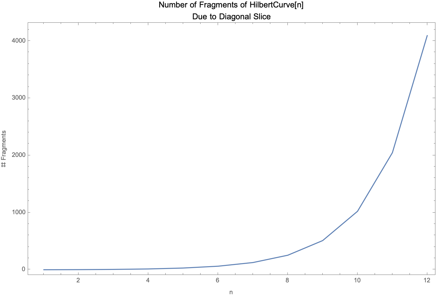
If this approximation is valid, we may be able guess the behavior of the true Hilbert curve by looking at how the number of intersections scales as we increase the index of the proto-Hilbert curve. This is easy enough to check in Mathematica, and we observe

HilbertCurveFragments.png

So the number of intersections does appear to be increasing with n (although, since the Hilbert curve is defined recursively, these computations quickly become intractable and difficult to check for n > 12). Does this mean that the true Hilbert curve is actually infinisected by the diagonal line? If I had to guess, I would guess that the answer is yes. But this is far short of a proof, and I have almost no idea how I would go about proving such a thing formally.

And if Hilbert curves solve our puzzle, what else does? Hilbert curves are not the only space-filling curves around. What about Peano curves?

PeanoCurve.png

I am not well-versed in the math of space-filling curves, but I am sure there are an infinite number of them. It would be very interesting to learn about the kinds of space filling curves which can be infinisected. Because the space filling curves that we have considered, exotic though they undoubtedly are, still have a sort of “regularity” to them. It is exciting to ponder what sort of bizarre, pathological, monstrously irregular (space-filling) curves might live out there in the Platonic world which could be infinisected if anyone could ever describe them.

A bizarre, pathological, monstrously irregular (approximation to a) space-filling curve.

A bizarre, pathological, monstrously irregular (approximation to a) space-filling curve.


At this point though, I have stepped far beyond my domain of expertise, so I will leave the post here. I hope you found this puzzle fun to think about. And again, if you can come up with other solutions, please post them in the comments! I would love to hear what people come up with.

Until next time, be well and be safe.

-Matt

Traveling the World

Lately, I’ve been having a lot of fun generating high-resolution satellite images of the Earth using Mathematica.

world.jpg

Mathematica has great built-in functionality for querying and manipulating satellite images, which I am just learning how to use. I generated this world map using

Screen Shot 2020-07-02 at 9.15.31 AM.jpg

The world is beautiful from this high up.


There is a famous problem in mathematics known as the Traveling Salesman problem. A traveling salesman must visit a number of cities. In which order should the salesman visit the cities so that he travels the least distance?

This question is of mathematical interest because, in the general case, it tends to be very difficult to solve. Technically, the Traveling Salesman problem is “NP-hard,” which means that finding a solution generally takes an exponential amount of computation. This is because the number of possible routes between the cities grows very quickly as you increase the number of cities.

However, for small numbers of cities, even an exponential amount of computation does not take too long. This means that we can actually solve the Traveling Salesman problem for many real-world scenarios. Suppose our salesman wants to visit all the world’s capitals. What route should he take?

Using Mathematica, this becomes quite easy to solve.

Screen Shot 2020-07-02 at 9.29.05 AM.jpg

That’s it! Here’s what it looks like (in high-res, of course!)

WorldTravelingSalesman.png

And here is the code I used to generate that image:

Screen Shot 2020-07-02 at 11.16.45 AM.jpg

We may not have solved the general Traveling Salesman problem, but I think this is a visually and conceptually interesting solution to a particular case.


Thank you for visiting my blog. As a statement of my affection and gratitude, I leave you with the Werner Projection...

Werner.png

The Period-Doubling Bifurcation Diagram

Hi friends,

Today, I would like to talk a bit about a particularly interesting result in chaos theory known as the Period-Doubling Bifurcation.

PeriodDoublingBifurcation4.png

I certainly don't know enough about this topic to explain it fully here, for it is a surprisingly deep and beautiful result. (For excellent explanations of the science surrounding this plot, see this video by Veritasium, and the book Chaos by James Gleick.) Instead, as my first attempt at understanding this bizarre beast, I wanted to illustrate how you produce the period-doubling bifurcation diagram. I hope to learn (and write!) much more about this in the future because I think it's fascinating. I hope you will agree!


The system we will consider is the logistic map, which is given by the simple recurrence relation:

logisticmap.png

Given some starting value x0, this equation allows you to compute x1. Then from x1, you plug back in and compute x2, and so on. Why would you ever want to do such a thing? As an example, the logistic map can be used as a primitive model of population growth. We say that x_n describes the current size of your population at time n. Then x_n+1 will describe the size of your population at time n+1. Two things to note: First, each x is between 0 and 1, so these population values should be thought of as the proportion of the maximum possible population. Second, r is a parameter of the system, so we can change r and get different population dynamics.

To make this concrete, let's choose a few values of r and see how our theoretical population evolves:

2.png
3.png
3_5.png
Several plots of population vs. time for different values of r in the logistic map. Note that all populations start with x0 = 0.25, but our ultimate results are robust to different initial values.

Several plots of population vs. time for different values of r in the logistic map. Note that all populations start with x0 = 0.25, but our ultimate results are robust to different initial values.

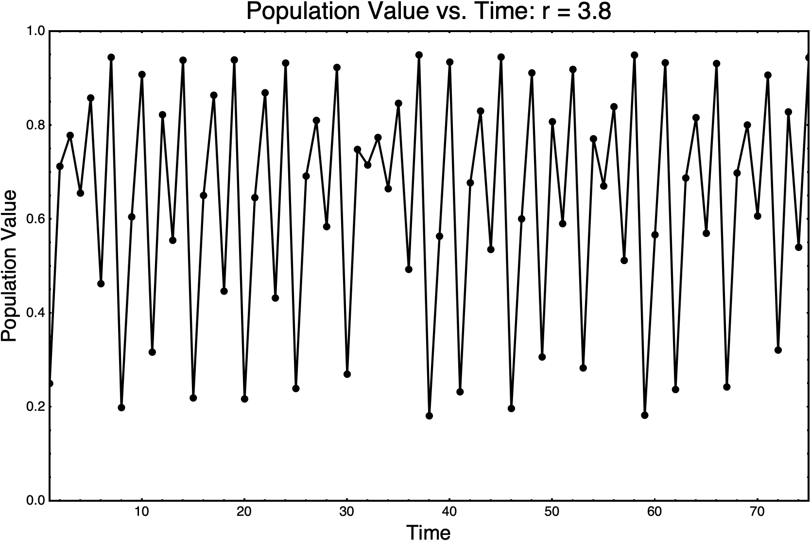
We can see that in some cases, the population quickly settles down to a nice equilibrium (r = 2). However, as we increase r, we can see that the population doesn't settle down to a single value. Indeed, in the case of r = 3.8, it does not appear to settle down at all. Here is what happens when we simulate r = 3.8 for longer.

Longer duration of population simulation for r = 3.8.

Longer duration of population simulation for r = 3.8.

So, let's see if we can quantify precisely how this steady-state behavior varies as we vary r. (By steady-state, I just mean we ignore the transient behavior at the beginning.)

After some initial amount of time, how many values does our population take, for a given value of r? In the case of r = 2 above, we see that the population takes on just a single value. For r = 3, it takes on two. And for r = 3.5, we would already have to count very carefully to see how many values it takes on. For r = 3.8, we would certainly want to count the steady-state values programmatically. To understand our results, we plot these steady-state values as a function of r, and derive the period-doubling bifurcation diagram.

PeriodDoublingBifurcation4.png

First and foremost, I think this is a beautiful plot. I certainly don’t claim to know everything that is going on here, but I find it absolutely mesmerizing to look at.

Here are a few simple observations about the period-doubling bifurcation diagram:

  • First, I find it extremely surprising that this much disorder and structure can be found in such a simple equation! (So did the people who discovered it, by the way!)

  • Second, there is not a simple trend from order to disorder in the plot. As you move along the r-axis, you get progressive bifurcations (i.e. splitting-in-twos) until the data seem completely disordered. And yet, there are definite pockets of relative order even after these points. I am not sure what causes the system to transition back to ordered behavior at these points.

  • Third, this diagram is actually self-similar. Looking closely at the first few bifurcations, you can begin to see that each is actually a slightly distorted copy of the whole structure

SelfSimilar1.jpg
SelfSimilar2.jpg
  • Fourth, there appear to be “threads” that extend through the whole diagram, even through the completely disordered regions. I also do not know how to make sense of these threads.

Close-up of “threads” that extend through regions of disorder in the bifurcation diagram.

Close-up of “threads” that extend through regions of disorder in the bifurcation diagram.

For me, one of the most surprising conclusions to be drawn from this plot is that real populations could exhibit highly complex dynamics from year-to-year or season-to-season, even with a very simple updating rule like the logistic map. One might have assumed that only simple behavior could occur in a system like this, but period-doubling shows that this is manifestly not the case!


I hope you found this interesting! I certainly did. If you would like to play with the code I used to create these images, feel free to download the notebook Bifurcations.nb from my GitHub page.

Thank you for reading!

-Matt

Volume of Spheres in Higher Dimensions

Hi everyone,

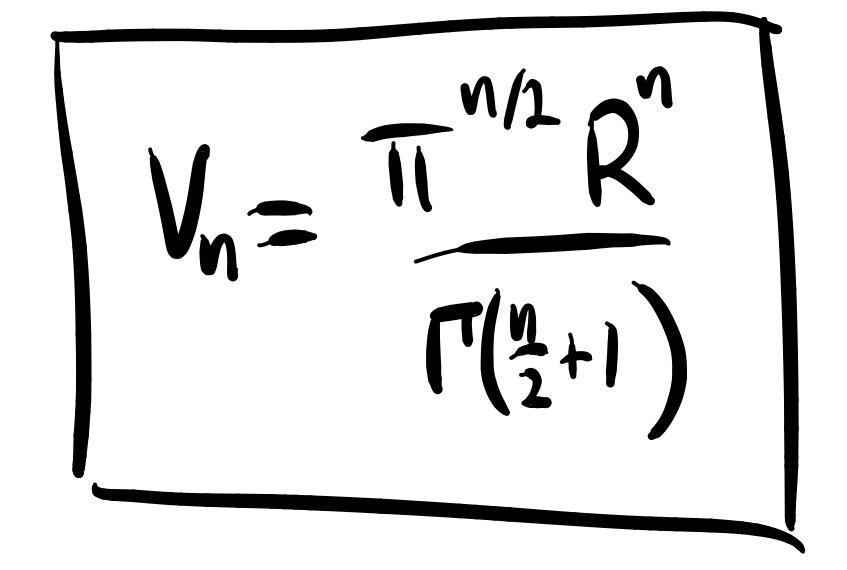
Today I will be deriving the formula for the volume of a sphere in any dimension. This is nothing new mathematically speaking, but it is exciting to me because I re-derived the results myself! Let’s get started.

Derivation

We define a sphere in n-dimensions as follows:

1.jpeg

We wish to compute the volume of this n-sphere, which amounts to computing the following integral:

2.jpeg

However, it is not immediately clear to me how to compute this integral given the irregular domain. Instead, we express the sphere as a function, and integrate this function to discover its volume. We choose the nth coordinate to be our function. That is,

3.jpeg

Note that we are now interested in the surface of the n-sphere, and we will integrate to find the volume enclosed by this surface.

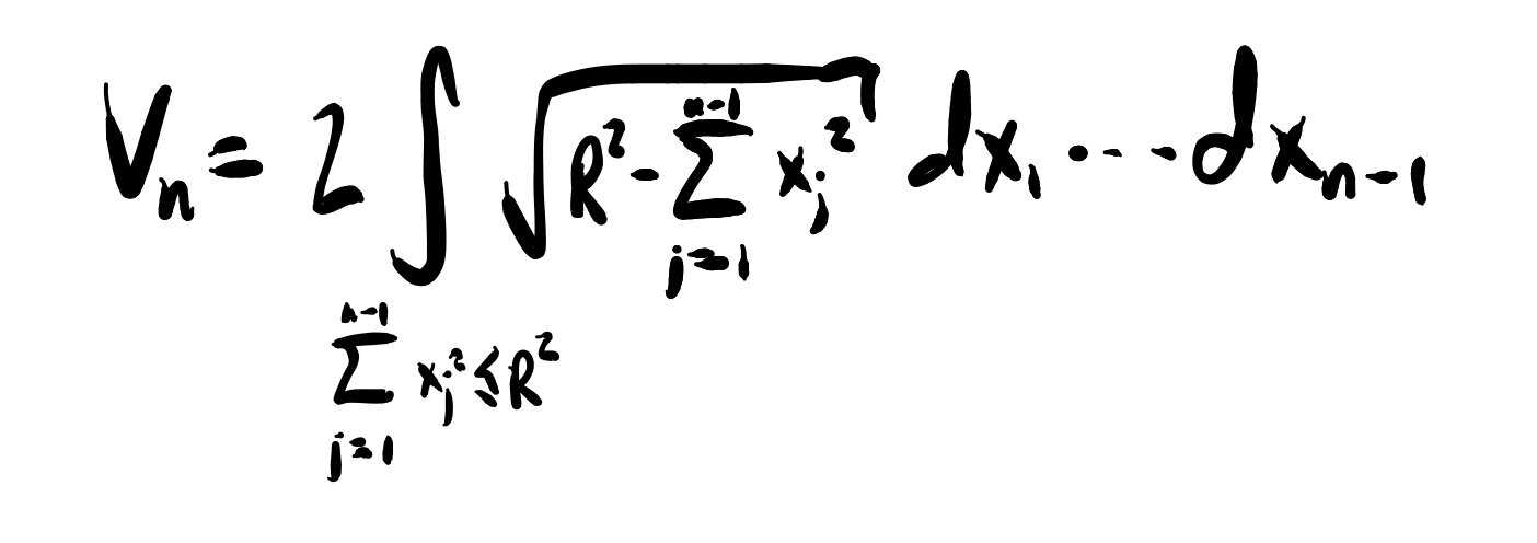
One issue that immediately presents itself is that this function is multivalued. We can address this in two ways. We could perform two integrals to get the volume enclosed by the positive part of the surface and the negative part of the surface respectively. Alternatively, we could recognize the symmetry between the positive and negative surfaces, find the volume underneath one of these surfaces, and then multiply our final answer by two. We choose the positive surface for convenience. Thus, we have

4.jpeg

Next, we must determine the bounds of this integral. They are going to be pretty ugly, given that we are still using cartesian coordinates. But we can at least write down the integrals somewhat easily in cartesian coordinates, and it turns out that we will actually be able to compute them with a little help from Mathematica.

Crucially, we observe that xn is now a function defined on the domain of {x1, …, xn-1}. That is, we are now integrating x_n over the (n-1)-sphere:

5.jpeg

At this point, I am going to take a second to define some notation. We are going to be writing expressions that look like what’s underneath the radical a lot, so let’s use the following shorthand:

6.jpeg

Next, we have to figure out the bounds of our integrals. We first integrate over the (n-1)-th variable. At this point, we have not constrained any of our other variables. So we will be integrating from one edge of the (n-1)-sphere to the other, which I claim amounts to

7.jpeg

I hope it is becoming clear why we introduced alpha. We next integrate the (n-2)-th variable. So far, we have integrated out x_n-1, but all the other variables remain to be considered. By the same logic, integrating the next variable across our (n-1)-sphere gives

8.jpeg

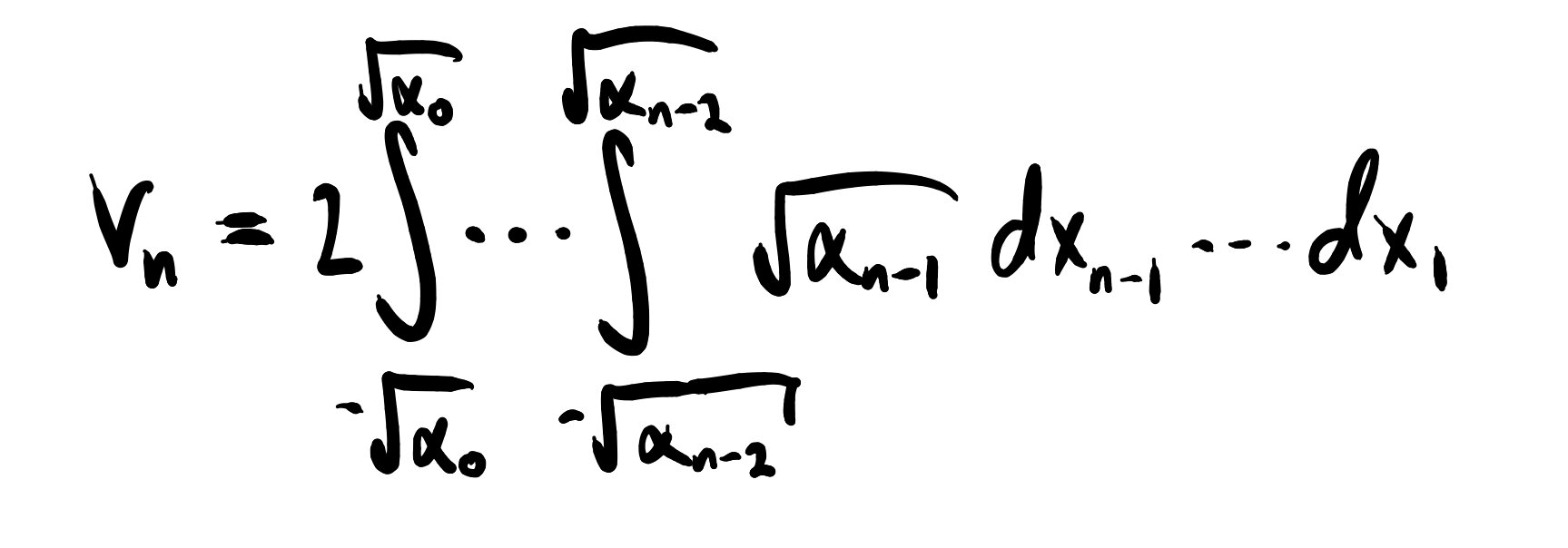
At this point, the pattern becomes clear. We simply continue this procedure until we have integrated over all our variables. We are now in a position to write down the full integral for the volume of a sphere in n-dimensions. Remembering our factor of 2 from earlier, we have

9.jpeg

Okay, it’s worth pausing at this point. This integral is very ugly, especially when we remember how much complexity we have subsumed into those alphas. Nevertheless, we now have a definite integral which contains our answer. If we can compute that integral, then we will have a general formula for the volume of a sphere in any dimension.

Well, it turns out that we actually can compute this integral, and we only need one result to do so. The result we need is as follows:

(integral computed in Mathematica)

(integral computed in Mathematica)

Now, let’s start working on our big nasty integral.

11.jpeg
12.jpeg
13.jpg

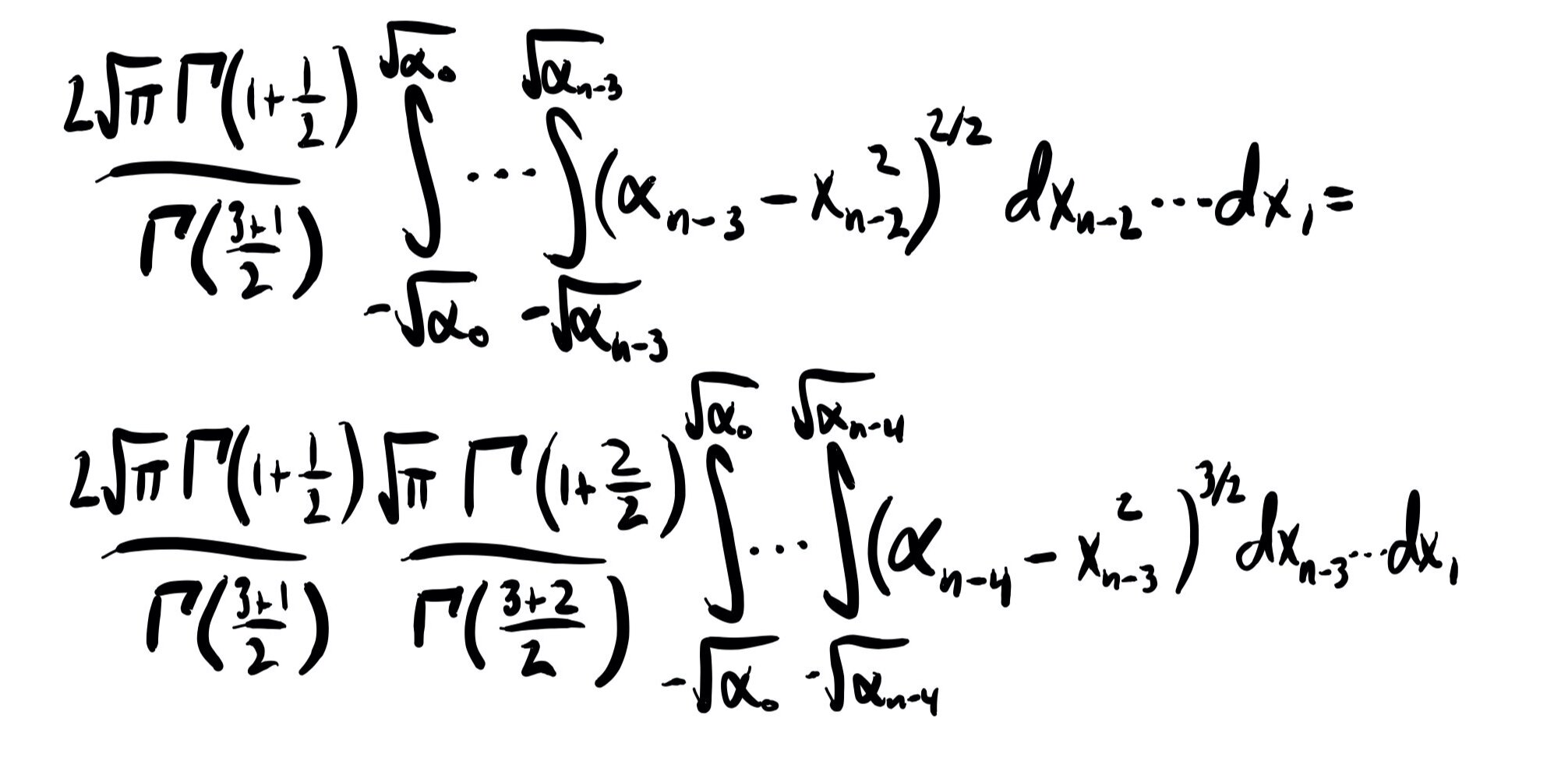
Here, we can start to see a pattern emerge. We will integrate each variable out one by one, each time acquiring a coefficient on the outside of the integral that depends on the exponent of the integrand, m. How long does this pattern continue? Until we run out of integrals. Since we integrate over n-1 variables, we will end up with coefficients

16.jpeg

Given that each integral simply increments the exponent on alpha by 1/2, we only need to evaluate the final integral to get our result:

15.jpeg

In fact, we already included the pi and gamma terms in the product we computed above, so all that we were missing was R^n. Finally, putting everything together, we derive the formula for the volume of a sphere in n-dimensions!

17.jpeg

Results and Discussion

I don’t blame you if you got lost in the above derivation. It certainly wasn’t the most elegant thing I’ve ever calculated. So I would like to make a few remarks on why I did it this way.

First of all, you may ask why I used cartesian coordinates to compute a result about spheres. And the answer is that I certainly tried to derive higher-dimensional spherical coordinates. I was able to derive the correct coordinates for dimensions 4 and 5. However, I was unable to come up with a systematic way of determining how the new angles I introduced were parameterized. Did they run from 0 to π? 0 to 2π? Did it vary based on the dimension? My naïve attempts to answer these questions gave me nonsense results for the volumes, so I had to find another way.

Second of all, you may ask why this was worth doing in the first place. This is a lot of calculus with a lot of square roots. What is the payoff? I claim that there is actually a big payoff for all that hard work. Let’s take a look at how the volumes of unit spheres (i.e. R=1) vary as we increase the dimension:

VolumeVsDimension.png

I don’t know what you were expecting, but I think that curve is astonishing. Who would have guessed that it would have a peak? It turns out that 5 dimensional unit spheres have the most volume! Naively, I would have guessed that they just kept getting bigger as you increase the dimension. And not only do they not keep getting bigger, but it is easy to verify that

18.jpg

Given that spheres are in some sense the simplest shape one can consider, it is clear that higher dimensions have many surprises in store indeed.

Elegant Little Plot

Here is a simple sequence that generates an elegant little plot.

Take each integer, and subtract from it the product of its decimal digits. When you plot the results, it looks like this:

IMG_2165.jpeg

While perhaps not the deepest result, it is aesthetically pleasing and extremely simple to program.

The script in Mathematica that generated this image was

points = {};

Do[AppendTo[points, n - (Times @@ IntegerDigits[n])], {n, 50000}];

ListPlot[points];

Although I have not given these structures much though, I’m fairly confident that the drooping features will occur just below multiples of 10. To see why, consider n = 999. The 999th element of the sequence will be 999-9^3 = 270. And yet, when n = 1000, the corresponding element of the sequence will be 1000-(1*0*0*0) = 1000. So the more 9’s (and less so 8’s, and even less so 7’s, and so on) a number has, the more will be subtracted.


This sequence, along with many other interesting ones, can be found at http://oeis.org, which is the Online Encyclopedia of Integer Sequences.

Functional Approach to the Catenary Problem

In this post, we will solve a famous problem in the history of physics: what shape does a chain take when it is hung between two posts?

Catenary7.png

In order to address this problem, we will make use of a so-called “functional” approach. That is, we will assign a functional for the potential energy of hanging chain, and we will try to find the shape of the chain that will minimize that energy.

First of all, we must define what a functional is. Simply put, a functional is a function which takes another function as its argument and returns a number. In this case, the function we are going to be using as our input will be the shape of the chain, y(x). Then, the functional will be a function that takes that shape function, and returns the chain’s potential energy. The fundamental question we wish to solve is: for which configuration of the chain, y(x), is our potential energy functional the smallest?

First, we must figure out how to write our functional in the first place. Typically, the gravitational potential energy of an object can be expressed simply as

Catenary3.png

However, we usually use this formula to describe the potential energy of a localized mass. In this case, we want to describe the potential energy of a spatially extended shape. So, what we will do instead is assign a potential energy for an infinitesimal segment of the chain, dU, and then integrate this over the length of the chain.

How can we find dU? We can get from the potential energy to an infinitesimal potential energy by replacing a point mass with an infinitesimal mass dm. We also change from y to y(x), to allow the height of the chain to vary from point to point along the chain.

Catenary8.png

If we wish to integrate over the length of the chain, we must then change our differential to be in terms of arc length along the chain. In this case, dm becomes

Catenary9.png

where mu is the mass per unit length along the chain (which we assume to be uniform), and ds is an infinitesimal segment of arc length.

Putting this all together, we finally have an expression for the total potential energy of the chain. Suppose that our posts are located at x = -L/2 and x = L/2. Then, the chain’s potential energy is given by

Catenary5.png

As a sanity check, is this actually a functional? Yes it is! It takes a function y(x) as an argument, and returns a number. So far so good.


At this point, we should pause and celebrate what we have done so far. It was not trivial to come up with this expression, and now that we have it, we are much closer to solving our problem. On the other hand, it appears that we have just hit a huge wall. We recall that our original goal was to find a configuration of the chain, y(x), that minimizes our potential energy functional. Taking a close look at this equation above should reveal that this is not such a simple thing to do.

At first we might propose simply taking a derivative of U with respect to y, and setting the result equal to 0. However, y(x) is an entire curve, not simply a variable. So the standard tools of calculus won’t be able to help us here. Luckily, there is technique from a branch of math known as the calculus of variations which allows us to sensibly take a derivative of U with respect to the entire function y(x). This operation is known as the variational derivative of U, or alternatively the functional derivative of U, and is denoted

Catenary10.png

So, we have now recast the catenary problem in terms of an equation involving a variational derivative: the configuration of the chain, y(x), which minimizes the potential energy U can be found by solving the equation

Catenary11.png

All that remains is figuring out how to solve this equation. Luckily, this is not so hard. All we need is one very important result from the calculus of variations.


Theorem: Suppose that we have a functional U, which is expressed in the following form

Catenary12.png

where script-L (often called the Lagrangian) is simply a function of x, y(x), and dy/dx. Then, the function y(x) which minimizes U with respect to y satisfies the Euler-Lagrange Equation:

Catenary13.png

It would take us too far out of our way to go through a proof of this theorem here. You can find one on the Wikipedia page, which I linked to above, if you are interested. In any case, proving this theorem is not necessary for understanding and using it. And this is a very important result in physics. Because many, many problems can reformulated in terms of minimizing functionals. And once we have done that, all we have to do is use this theorem, and then we can find their solutions.

So let’s find the catenary curve!

If we compare the general formula given in the theorem with the specific one that we derived, we see that our Lagrangian is given by

Catenary14.png

Given that we wish to minimize the potential energy with respect to y, we must now plug into the Euler-Lagrange equation. Doing so will allow us to find y(x). What follows is a lot of messy calculus, so strap in.

Catenary15.png

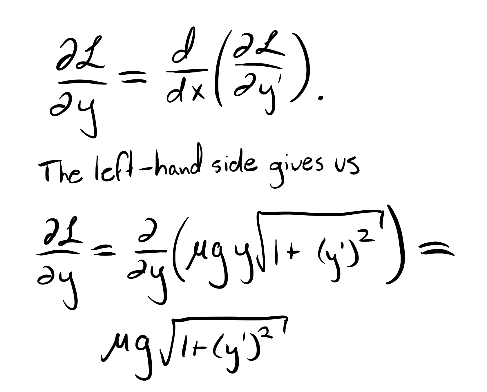
It is important to note here that, when solving the Euler-Lagrange equation, y and y’ are treated like two entirely separate variables! This is why the square root term is not affected by this partial derivative.

Catenary16.png
Catenary17.png

(I forgot my mu • g! I will put it back I promise.)

Catenary18.png

We now equate the two sides of the Euler-Lagrange Equation, put back the mu and g where they are supposed to go, and get

Catenary19.png
Catenary20.png

Whew! Okay, let’s take a breath, and examine what we got. That was certainly a mess, but it was really just taking a few particularly nasty derivatives. Now that we have done so, we are left with a differential equation for y. If we can solve that differential equation, we will have found the shape of our chain, at long last.

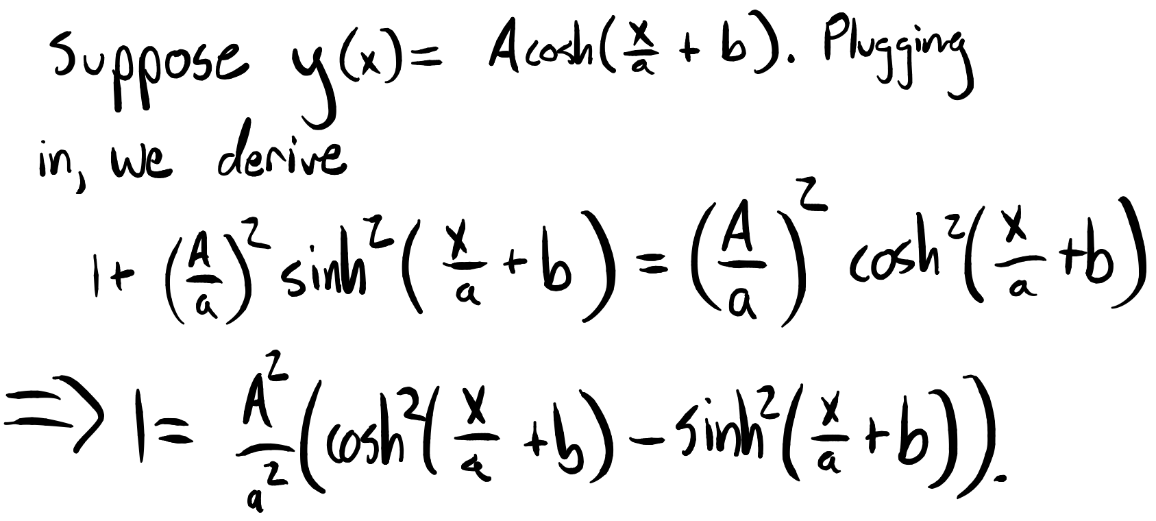
Unfortunately, this equation is nonlinear, so you won’t get anything nice by simply plugging into your favorite differential equation solver. However, it is not too difficult to simply guess what a nice solution might be, and see what we get. If you throw solutions against the wall for long enough, you might propose the following:

Catenary22.png

Lastly, we recall that we imagined our chain to be hung between posts at x = -L/2 and x = L/2. As a result, the chain will be symmetrical about x = 0. Since cosh(y) is symmetrical about x = 0, we conclude b = 0. Thus, we arrive at our final answer:

Catenary23.png

(Interjection from future Matt!!! You might, like me, have found the solution to the differential equation above a bit unsatisfying. I was not up to the task of solving it myself, but my good friend Jeremy Welsh-Kavan found and wrote up a great solution. Check it out here.)

This is known as the catenary curve! Below, I have plotted the catenary curve for different values of a, with the fence posts at x = ± 3.

Catenary27.png

The last thing that remains is to compare it with a real hanging chain.

Catenary26.JPG

Not a bad fit!